CEEn 414 - Civil Engineering Applications of GIS

Groups
 

Account Login

Overview
Liquefaction Index (LI)
Data Requirements
Output
Data Preparation
Analysis Methodology in GIS
Assignment Outline
 

Overview

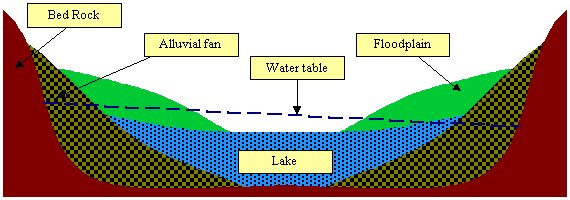
Liquefaction is a major cause of damage associated with earthquakes.  While liquefaction is a complex phenomenon, a simplified model can help to predict regions of high and low susceptibility.  Knowing where there is a  high potential for liquefaction to occur can help developers and designers take necessary precautions to minimize risks against life and property.

Locations most vulnerable to liquefaction and lateral spread lie near river channels or on gently sloping ground that is underlain by loose water-saturated granular sediments.  In this project we will use soil layer depths, water table depth, and percentage of liquefiable soils to develop a liquefaction susceptibility index map.  While there are numerous classes of soils, we will consider only three in our model: 1) Lake deposits, 2) Alluvial fan deposits, and 3) Flood plain deposits.  The bedrock layer will provide the lower boundary as well as the extents of the model.  The figure below illustrates generally how these three types of sediments might interact with each other.  In addition to these data layers we will also use borehole samples that indicate a percentage of liquefiable soils at that location to develop our map.  The following paragraphs outline the process by which a liquefaction index map can be generated from these data using a GIS.

Notes:
1) The extent of bed rock surface represents the extent of analysis.
2) The top elevation of rock surface is the lowest possible elevation of the bottom surface of any liquefiable layer.

Liquefaction Index (LI)

The liquefaction potential index (LI) is the total liquefiable depth of all available layers at any particular location.

    LI = (Ds * Lp / 100)_Layer1  +  (Ds * Lp / 100)_Layer2  + (Ds * Lp / 100)_Layer3 + ........

    where,
    LI     =    Liquefaction Index
    Ds    =    Saturated soil depth
    Lp    =    Percent of Liquefaction

The saturated depth (Ds) is obtained by comparing the water table elevation with the top and bottom surface elevations of a given layer. The percent of liquefaction (Lp) is obtained from borehole test results. The Lp essentially represents the percentage of the saturated depth that could potentially liquefy under adverse conditions.

Data Requirements

The top surface elevation of the following geologic materials and water table are in grid format.  This particular assignment is done using "contrived" data.  However, you could create these grid files for a separate analysis using borehole log information and then interpolating similar to the way in which we will create the percent liquefiable grids below.  All data are in the UTM NAD 27 Zone 12 (meters) projection, but their projections have not yet been defined and so you will want to do this before proceeding with the actual analysis.

    Material        GridName            Comment
1. Bed Rock       Rock                    Serve as the datum. Not liquefiable.
2. Alluvial Fan    AFan                    Liquefiable
3. Lake              Lake                     Liquefiable
4. Floodplain      FPlain                   Liquefiable
5. Water table    WTable                Used to determine the saturated depth.
 

Borehole locations and percent of liquefaction of all liquefiable layers in shapefile format.  Like the grids, the borehole data are also in the UTM NAD 27 Zone 12 projection, but no .prj file is included and so you will want to define the projection before doing the analysis.

Shapefile: Bore.shp

    Attribute           Description
1. IAFan                Percent liquefaction of the alluvial fan.
2. ILake                 Percent liquefaction of the lake materials.
3. IFPlain                Percent liquefaction of the floodplain.

You can download the five grids and borehole shape file by clicking here.

Output

The result of the analysis will be a single grid (LIndex)  representing the Liquefaction Index (LI) over the entire area.

Data Preparation

Create the "Percent Liquefaction (Lp)" grid for each liquefiable layer from the borehole data (Bore.shp).  You will need to use the spatial analyst and interpolate the borehole data to create the three different grids for each of the three soils layers.

    Attribute of Bore.shp       
1. IAFan    Percent liquefiable fines in the alluvial fan layer                              
2. ILake     Percent liquefiable fines in the lake sediments layer                               
3. IFPlain   Percent liquefiable fines in the flood plain layer                          

Analysis Methodology in GIS

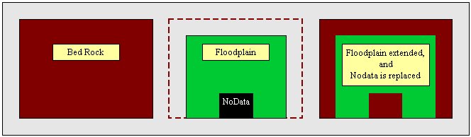
1)  Changing the extent and replacing NoData

In grid analysis, the NoData areas in any input grid become NoData areas in the output grid. Therefore, in order to obtain a continuous liquefaction index surface over the entire analysis domain we need to eliminate NoData areas from all liquefiable layers (alluvial fan, lake, and floodplain). This is done by "merging" the rock layer with each of the liquefiable layers. In this case, the "merge" operation does two things, 1) it replaces the no data area, and 2) it also extends the boundary. The result of a "merge" operation is illustrated in the following figure.  For more information on using the Merge command click here. 

You will input the upper elevation grid of each layer and merge them separately with the rock layer. 

You are starting to create a lot of grids now so be sure you manage them appropriately (for example after merging the original flood plain (alluvial fan, lake, water table) grid with the bedrock you will want to eliminate the original in favor of the new flood plain grid that has the full extents and no data areas eliminated so that you do not become confused later on.

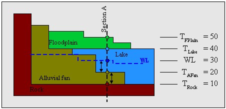
2) Determining the bottom elevation of each liquefiable layer

The bottom surface elevation of any liquefiable layer is the top surface elevation of the underlying layer. In the figure, the floodplain material is lying on alluvial fan  in the left side and extended over the lake on the right side. Which means the bottom surface elevation of the floodplain layer depends on the alluvial fan layer in some areas, and on the lake layer in others. Therefore, the bottom surface elevation of any layer must be obtained by comparing ALL possible underlying layers and determining the "next" top elevation. The following example illustrates the procedure, though keep in mind that it is ONE cross section and that your analysis is done over the entire domain and hence why you need to consider comparison against all layers and not go just by what you see in this one cross section.

Let's say, we want to determine the bottom surface elevation of floodplain layer (B_FPlain)  at section A. Since we know that the top surface elevation of rock is the lowest possible bottom surface elevation for any layer, the first assumption would be  B_FPlain= T_Rock.. Then we we will compare this value with the top surface elevation of other layers.

Trial 1: B_FPlain= T_Rock= 10.

Trial 2: Compare with  the lake layer.
- T_Lake is lower than T_Fplain ,  therefore, it is an underlying layer at that section and is a possibility.
- T_Lake (= 40) is higher than B_FPlain (= 10) obtained in trial 1, therefore, we set B_FPlain= T_Lake= 40.

Trial 3: Compare with the alluvial fan layer.
- T_AFan is lower than T_Fplain, therefore, it is an underlying layer at that section and is a possibility.
- T_AFan (= 20) is lower than B_FPlain (= 40)obtained in trial 1, therefore, we discard this value and  B_FPlain remain same as before.

The final B_FPlain= T_Lake= 40.

If we do this operation for each grid cell in our grid we can derive a bottom layer grid for the flood plain.  We then repeat this process for each of the other two liquefiable layers (lake, and alluvial fan).

3) Determining the saturated depth of each liquefiable layer

The saturated depth (Ds) is the depth of any layer under water at any particular section (grid cell). This is obtained by comparing the water table elevation with top and bottom surface elevation of a liquefiable layer. For each grid cell, one of three possibilities exist: 1) the water lever can be above the top elevation, 2) in between the top and bottom elevations, or 3) below the bottom elevation.  Let's say, we want to determine the saturated depth for each layer at section A as shown in the following figure.

Floodplain:
WL (=30) is below the bottom surface elevation (case 3), therefore, the saturated depth is zero. (Ds_FPlain = 0)

Lake:
WL (=30) is above the bottom surface elevation but below the top surface elevation (case 2), therefore, the saturated depth would be the difference between the water table and the bottom surface elevation. Ds_Lake = WL - B_Lake = 30 - 20 = 10.

Alluvial fan:
WL (=30) is above the bottom surface elevation and also above the top surface elevation (case 1), therefore, the saturated depth would be the difference between the top and the bottom surface elevation. Ds_AFan = T_AFan - B_AFan = 20 - 10 = 10.

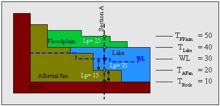
This operation is performed using the Con function in Spatial Analyst.  For more information on using Con to perform this operation click here.

4) Creating the Liquefaction Index (LI) grid (LIndex)

The liquefaction potential index (LI) is the total liquefiable depth of all available layers at any particular site.

    LI = (Ds * Lp / 100)_Layer1  +  (Ds * Lp / 100)_Layer2  + (Ds * Lp / 100)_Layer3 + ........

Let's compute LI at section A as shown in the following figure.

    LI_A = (Ds * Lp/ 100)_FPlain  +  (Ds * Lp / 100)_Lake  + (Ds * Lp / 100)_AFan
or LI_A = (0 * 25 / 100)_FPlain  +  (10 * 35 / 100)_Lake  + (10 *15/ 100)_AFan
or LI_A = 5

Assignment Outline

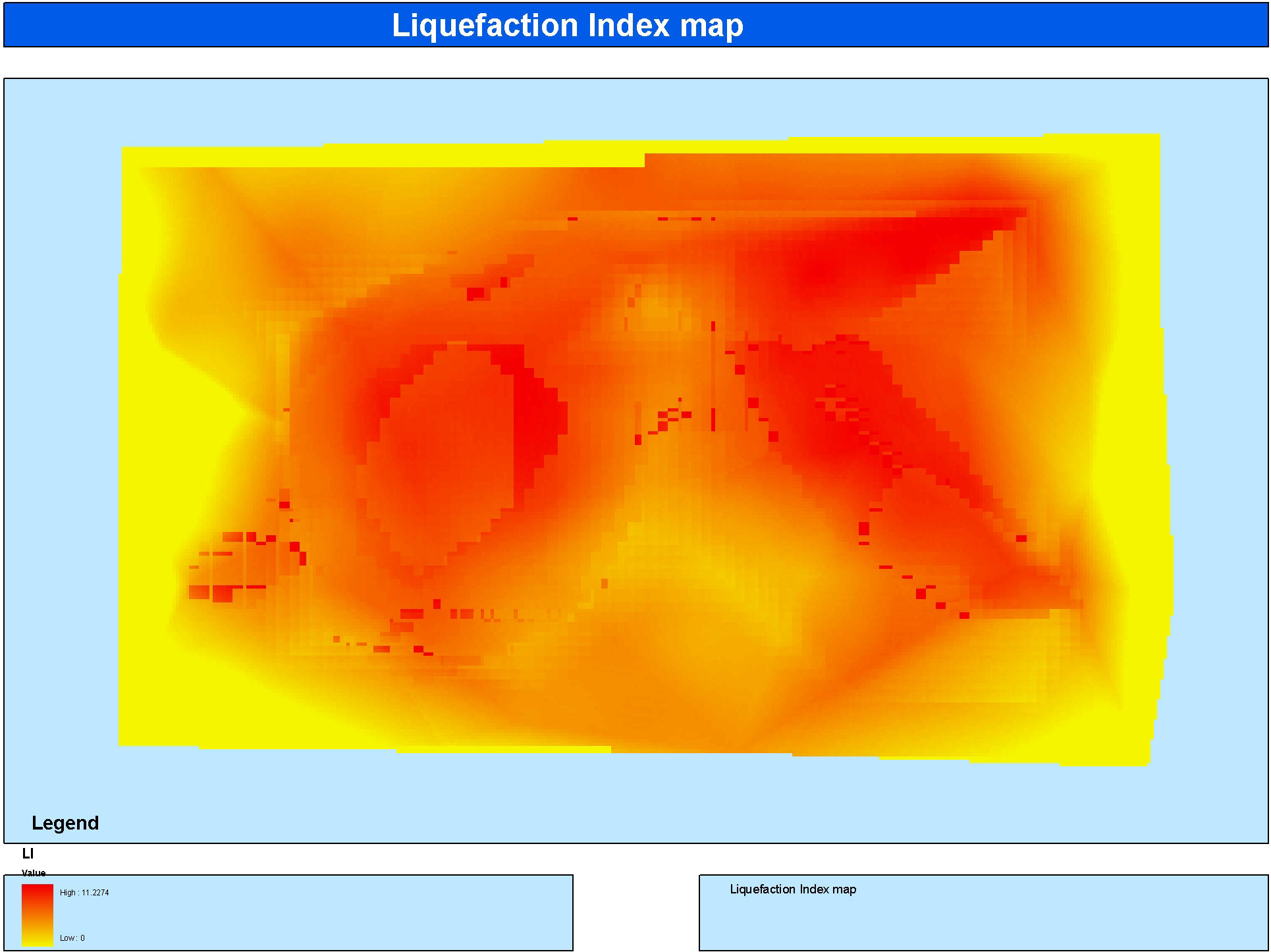
Create a report as part of a web page (one per group is fine, but each person should Email the TA in order to get credit) that includes a layout map showing your resulting liquefaction map for the given data.

Included in your report you should also outline the steps you used to create your map using the model builder as an outline of how you solved the problem.

Basic Outline

Data Preparation
Project the data, interpolate the boreholes to rasters (use the bedrock extents and cell size)

Change the extent of the grids and replace NoData area with rock surface elevation

Determine the bottom elevation of each liquefiable layer

Determine the saturated depth of each liquefiable layer

Create Liquefaction Index (LI) grid (LIndex)
 

Email the TA when you are finished.